How to sort and filter data in Excel

Sorting and filtering data offers a way to reduce noise and find (and sort) only the data you want to see. Microsoft Excel has no shortage of options for filtering huge data sets into what’s needed.

How to Sort Data in an Excel Spreadsheet

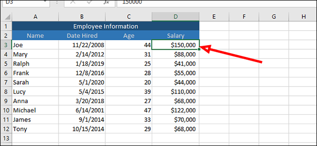
In Excel, click inside the cell above the column you want to sort by.

In our example, we’re going to click on Cell D3 and sort this column by salary.

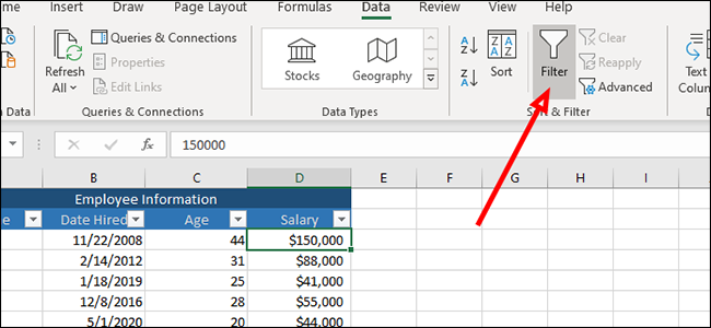
From the “Data” tab at the top of the ribbon, click “Filter.”

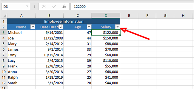
Above each column, you will now see an arrow. Click on the arrow of the column you want to sort to open a menu that allows us to sort or filter the data.

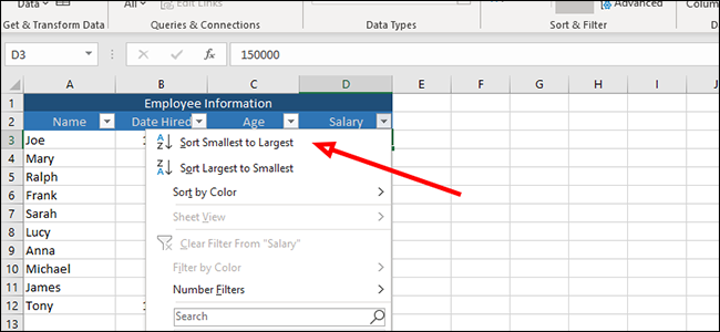
The first and most obvious way to order data is smallest to largest or largest to smallest, assuming you have numeric data.

In this case, we’re ranking salaries, so we’d like to sort from smallest to largest by clicking the top option.

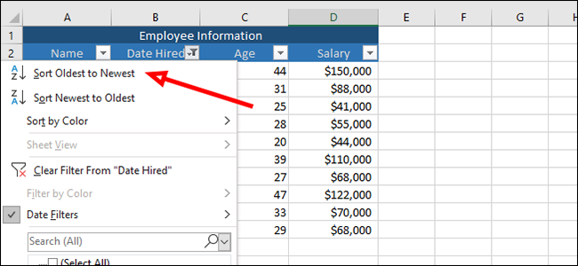
We can apply the same sort to any of the other columns, sorting by rental date, for example, by selecting the “Sort Oldest to Newest” option in the same menu.

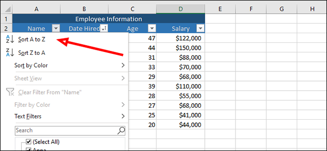
These sort options also work for the age and name columns. We can sort oldest to youngest age, for example, or organize employee names alphabetically by clicking the same arrow and choosing the appropriate option.

How to filter data in Excel

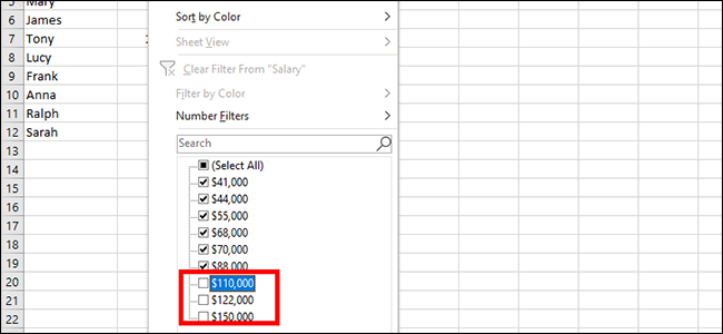
Click the arrow next to “Salary” to filter this column. In this example, we’re going to filter out anyone who makes more than $100,000 per year.

Because our list is short, we can do this a couple of ways. The first way, which works great in our example, is just to uncheck each person who makes more than $100,000, and then hit “OK.” This will remove three entries from our list and allow us to view (and sort) only those that remain.

There is another way to do this. Let’s click the arrow next to “salary” one more time.

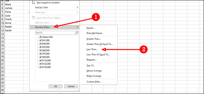
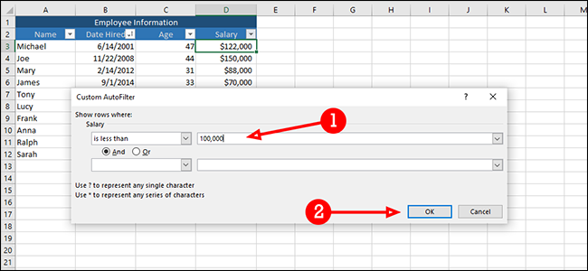
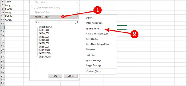
This time, we’ll click on “Numeric Filters” in the Filtering menu and then “Less Than”.

Here we can also filter our results, removing anyone who has greater than $100,000 per year. But this way works much better for large datasets where you may have to do a lot of manual clicking to remove entries. To the right of the drop-down box that says “is less than,” enter “100,000” (or whatever you want to use) and then press “OK.”

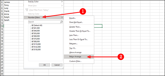
We can also use this filter for various reasons, too. For example, we can filter all salaries that are above average by clicking “below average” in the same menu (Number and GT Filters; below average).

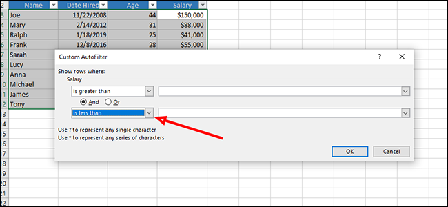
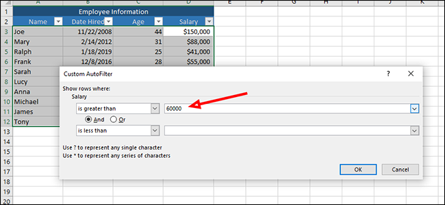
We can also combine filters. Here we will find all salaries above $60,000, but less than $120,000. First, we’ll select “is greater than” in the first dropdown box.

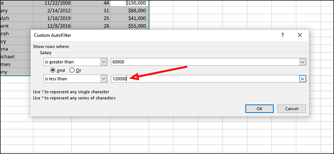
In the dropdown below the above, choose “is less than”.

Next to “is greater than” We’ll put in $60,000.

Next to “is less than” add $120,000.

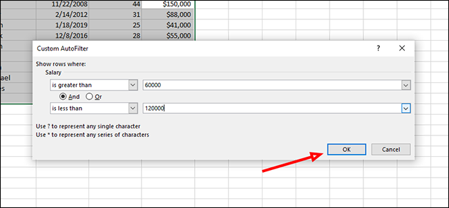
Click “OK” to filter the data, leaving only salaries greater than $60,000 and less than $120,000.

How to filter data from multiple columns at once

In this example, we are going to filter by date hired and salary. We’ll look at it specifically for people hired after 2013, and with a salary of less than $70,000 per year.

Click the arrow next to “Salary” to filter out anyone making $70,000 or more per year.

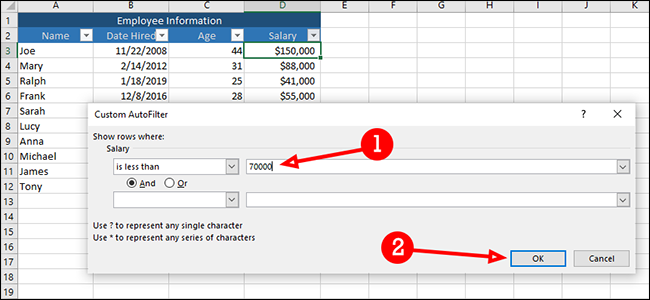
Click on “Numerical Filters” and then “Less Than”.

Add “70,000” next to “is less than” and then press “OK”.

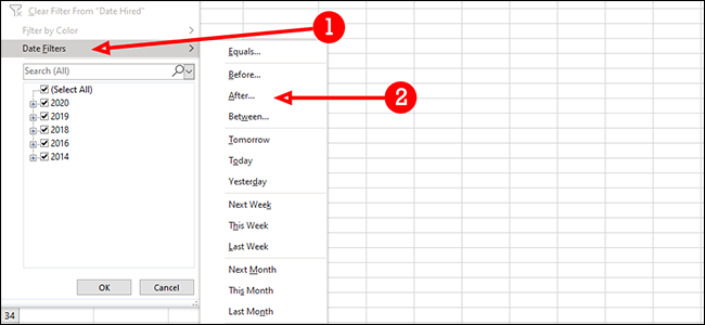
Next, we’re going to filter by the date each employee was hired, excluding those hired after 2013. To get started, click the arrow next to “Date Hired” and then choose “Date Filters” and then “After “.

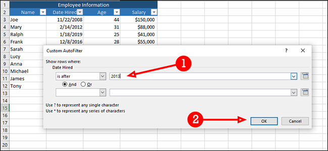
Type “2013” in the field to the right of “is after” and then press “OK.” This will leave you with only employees who make less than $70,000 per year, and were hired in 2014 or later.

Excel has a number of powerful filtering options, and each one is as customizable as you’d need it to be. With a little imagination, you can filter down huge data sets to just the pieces of information that matter.